CRD cookbook

Author

Kanth JS

Published

November 2, 2025

CRD version update in 2025

#TL;DR:
CRD ปี 2025 การรายงานควรที่จะแสดง “ค่าประมาณ + 95% CI” และขนาดเอฟเฟกต์ (η²/ω²) มากกว่าดูจากค่า p-value อย่างเดียว นะ

เกริ่น

ตั้งใจ ทำ การวิเคาะห์ข้อมูลการทดลองที่ออกแบบ CRD แบบที่คิดว่าสมบูรณ์ที่สุด รวบรวมมากจากทุกที่ โดยพยายามจะอัพเดท การวิเคราะห์ที่ทันสมัยให้มากที่สุด ในปี 2025

# packages
pacman::p_load(
  tidyverse, # data import and handling
  conflicted, # handling function conflicts
  emmeans,
  multcomp,
  multcompView, # adjusted mean comparisons
  ggplot2,
  effectsize, # effect size calculation
  desplot, # for plotting experimental designs
  rstatix,
  ggdist,
  performance,
  see
) # plots

package 'rstatix' successfully unpacked and MD5 sums checked

The downloaded binary packages are in
    C:\Users\sithj\AppData\Local\Temp\RtmpMnOMHd\downloaded_packages

# conflicts between functions with the same name
conflict_prefer("filter", "dplyr")
conflict_prefer("select", "dplyr")

Data

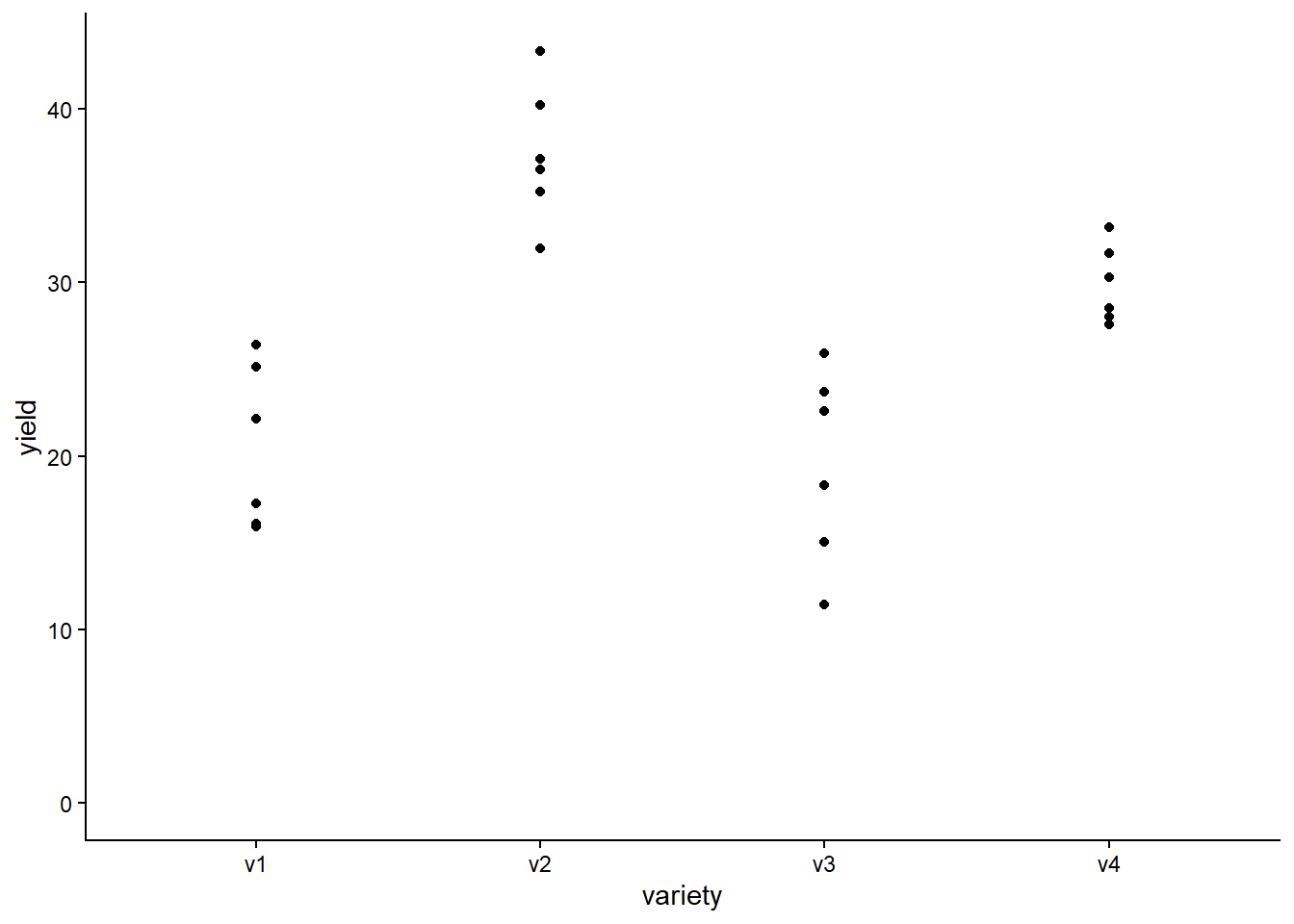
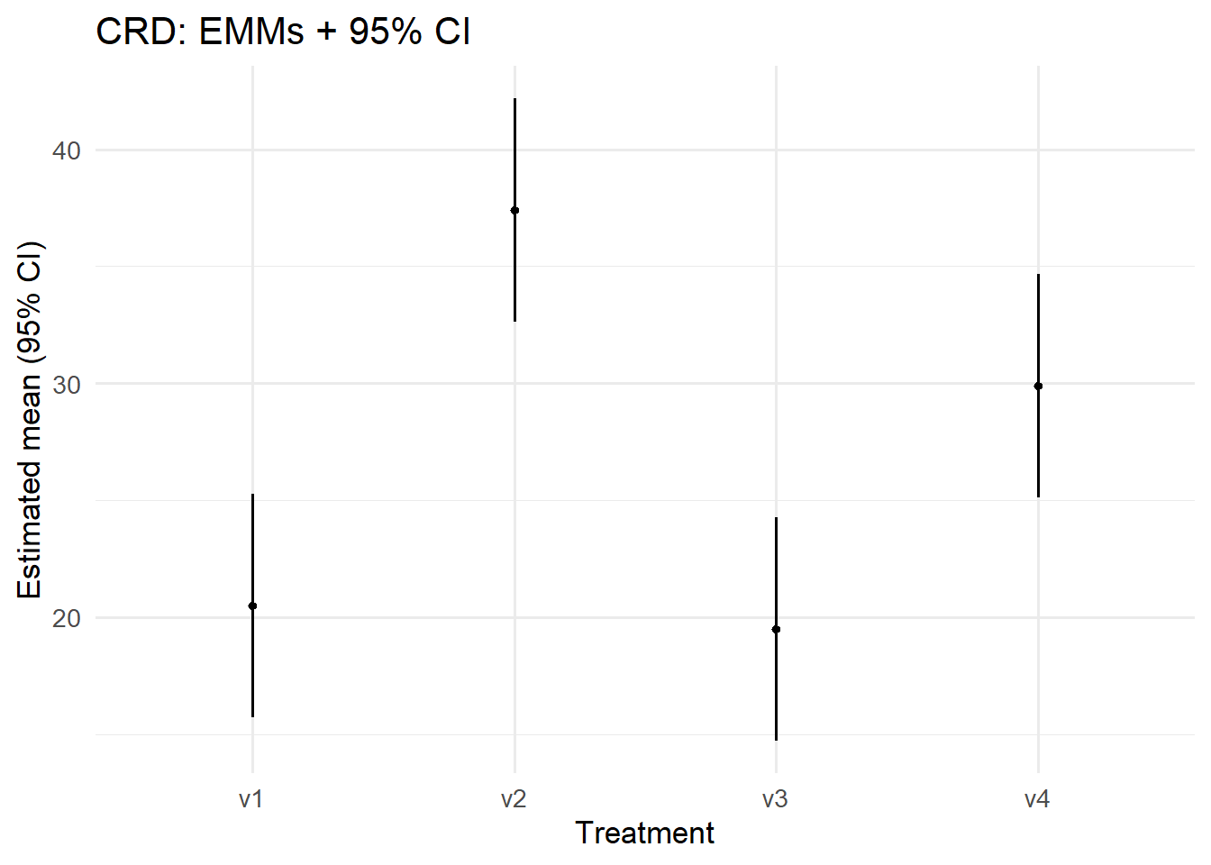
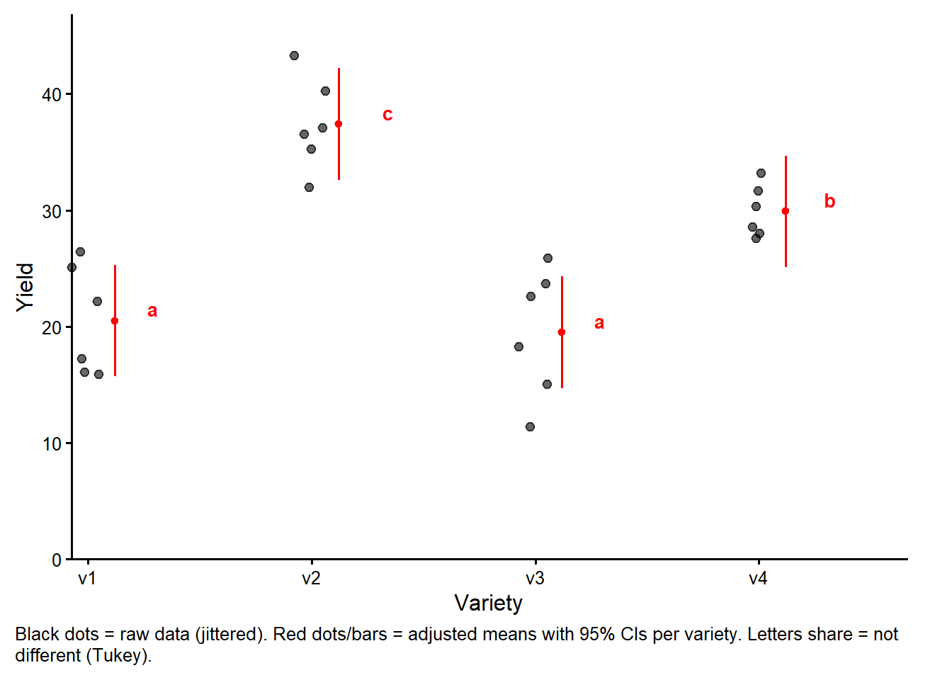
ข้อมูลที่มาทำได้เป็นงานวิจัยทดสอบผลผลิตเมลอน ตีพิมพ์ Mead et al. (1993, p.52) โดยการทดลองมีพันธุ์เมลอน 4 พันธุ์ แต่ละพันธุ์ได้รับการทดสอบในแปลงทดลองจำนวน 6 แปลง ออกแบบการทดสอบแบบ สุ่มสมบูรณ์ (CRD) จาก “Example 4.3” หนังสือ “Quantitative Methods in Biosciences (3402-420)” by Prof. Dr. Hans-Peter Piepho

Import and wrangle data

dataURL <- "https://raw.githubusercontent.com/SchmidtPaul/DSFAIR/master/data/Mead1993.csv"
dat <- read_csv(dataURL)
dat %>% head()

variety	yield	row	col
v1	25.12	4	2
v1	17.25	1	6
v1	26.42	4	1
v1	16.08	1	4
v1	22.15	1	2
v1	15.92	2	4

แล้วเราจะยังต้องทำให้ตัวแปรต้นของเราเป็น factor เสียก่อนจึงจะถูกต้อง

dat <- dat %>% mutate(across(variety, as.factor))

มาดู ข้อมูลผลผลิตกันก่อนว่าเป็นอย่างไรในเมลอนแต่ละพันธุ์

ggplot(data = dat, aes(y = yield, x = variety)) +
  geom_point() + # scatter plot
  ylim(0, NA) + # force y-axis to start at 0
  theme_classic() # clearer plot format

จากตรงนี้ก็พอจะเห็นอะไรบ้างว่า มีพันธุ์บางพันธุ์นั้น มีผลผลิตต่างกัน ต่อไป มาวิเคราะห์ ANOVA กัน

Modern ANOVA = `car::Anova(type = 3)`

fit <- lm(yield ~ variety, data = dat)
car::Anova(fit, type = 3)

	Sum Sq	Df	F value	Pr(>F)
(Intercept)	2519.0406	1	137.0335	0e+00
variety	1291.4771	3	23.4184	9e-07
Residuals	367.6531	20	NA	NA

ถ้าเป็น code แบบ classic ก็ใช้ aov(yield ~ variety, data = dat) ซึ่ง ถ้าเป็น ปัจจุบันตอนนี้ เราจะนิยมและปลอดภัยสุด หรือ ANOVA type จาก Data Science for Agriculture in R

In most cases it’s probably best to conduct a Type III ANOVA, e.g. via car::Anova(model, type = "III").

classic ANOVA

แบบ ANOVA จาก R base ก็ใช้ได้เช่นกัน นะ

aov.model <- aov(yield ~ variety, data = dat)
summary(aov.model)

            Df Sum Sq Mean Sq F value   Pr(>F)    
variety      3 1291.5   430.5   23.42 9.44e-07 ***
Residuals   20  367.7    18.4                     
---
Signif. codes:  0 '***' 0.001 '**' 0.01 '*' 0.05 '.' 0.1 ' ' 1

ถ้า ไม่ sig เราก็ จะรายงาน เท่านี้ แต่ถ้าไม่ ส่วนใหญ่ เราก็จะไปทดสอบต่อ อย่างที่เรา เรียกกัน postpoc

ตรวจ Asusumption

ใช้ performance library หรือ easystat library เพื่อ check สมมุติฐาน และคุณภาพของข้อมูล ที่นำไปวิเคราะห์ ANOVA

Homogeneity check

performance::check_homogeneity(fit)

OK: There is not clear evidence for different variances across groups (Bartlett Test, p = 0.314).

performance::check_homogeneity(fit) %>% plot()

heteroscedasticit check

performance::check_heteroscedasticity(fit)

OK: Error variance appears to be homoscedastic (p = 0.233).

performance::check_heteroscedasticity(fit) %>% plot()

บอกว่าต้องเชคอันนี้ก่อน เพราะว่ามันจะมีผลต่อ การวิเคราะห์ ANOVA เพราะว่า ถ้าไม่ ก็ ควรใช้ Welch ANOVA แทน

Normality check

performance::check_normality(fit)

OK: residuals appear as normally distributed (p = 0.619).

performance::check_normality(fit) %>% plot()

หลายคนอยากดู outlier

check_outliers(fit) %>% plot()

ขนาดเอฟเฟกต์

อยากจะชวนให้ ดู effect ต่อ สำคัญอย่างไร - p-value บอกแค่ว่า “มีหลักฐานต่างกันไหม” ซึ่งไวต่อ ขนาดตัวอย่าง มาก แต่ ไม่บอกว่าผลที่ได้นั้นต่างกันมากขนาดไหน - ขนาดเอฟเฟกต์บอก “ผลที่ได้ใหญ่พอจะมีความหมายเชิงปฏิบัติไหม” และทำให้ เปรียบเทียบงาน/การทดลองต่างกันได้ บนมาตรฐานเดียว

effectsize::eta_squared(fit)

Parameter	Eta2	CI	CI_low	CI_high
variety	0.7784061	0.95	0.5957645	1

effectsize::omega_squared(fit)

Parameter	Omega2	CI	CI_low	CI_high
variety	0.7370013	0.95	0.5243762	1

ค่า omega square (variance explained): “ทรีตเมนต์อธิบายความแปรปรวนได้ ~73% (ω²=0.73) ผลต่างเห็นได้ชัด (รู้สึกมั่นใจว่าผลการทดลองที่ได้สังเกตเห็นผลต่างได้ชัดเจน)”

post-hoc test

แม้ปัจจุบัน นักสถิติหลายคน ไม่ค่อย สนับสนุนให้ ทำ CLD(compact letter dusplay) เพราะว่า … แล้ว แต่ในสาขาเกษตรหรือชีววิทยา ก็ยังคงนิยมเพระาว่า ง่ายในการอธิบายผล ดังนั้น เราจะยังใช้

ประมาณค่าเฉลี่ยเปรียบเทียบ โดยการใช้ตัวอักษร

emm <- emmeans(fit, ~variety)
contrast(emm, "pairwise", adjust = "tukey")

 contrast estimate   SE df t.ratio p.value
 v1 - v2   -16.913 2.48 20  -6.833  <.0001
 v1 - v3     0.998 2.48 20   0.403  0.9772
 v1 - v4    -9.407 2.48 20  -3.800  0.0057
 v2 - v3    17.912 2.48 20   7.236  <.0001
 v2 - v4     7.507 2.48 20   3.033  0.0307
 v3 - v4   -10.405 2.48 20  -4.203  0.0023

P value adjustment: tukey method for comparing a family of 4 estimates

ตารางข้างบ้นนี้ เปรียบเทียบทีละคู่ ๆ

เปรียบเทียบโดยการใช้ตัวอักษร CLD

mean_comparisons <- fit %>%
  emmeans(specs = "variety") %>%
  cld(adjust = "tukey", Letters = letters)

mean_comparisons

	variety	emmean	SE	df	lower.CL	upper.CL	.group
3	v3	19.49167	1.750365	20	14.70324	24.28009	a
1	v1	20.49000	1.750365	20	15.70158	25.27842	a
4	v4	29.89667	1.750365	20	25.10824	34.68509	b
2	v2	37.40333	1.750365	20	32.61491	42.19176	c

กราฟเปรียบเทียบตัวแปร

ggplot(mean_comparisons, aes(variety, emmean)) +
  ggdist::geom_pointinterval(
    aes(ymin = lower.CL, ymax = upper.CL)
  ) +
  labs(
    x = "Treatment",
    y = "Estimated mean (95% CI)",
    title = "CRD: EMMs + 95% CI"
  ) +
  theme_minimal(base_size = 13)

my_caption <- "Black dots = raw data (jittered). Red dots/bars = adjusted means with 95% CIs per variety. Letters share = not different (Tukey)."

ggplot() +
  aes(x = variety) +

  # จุดดิบ: jitter ป้องกันทับกัน + alpha ให้โปร่ง
  geom_point(
    data = dat,
    aes(y = yield),
    position = position_jitter(width = 0.08, height = 0),
    alpha = 0.6,
    size = 1.9
  ) +

  # ค่ากลางและช่วงเชื่อมั่น (ใช้ pointrange แทน point + errorbar แยก)
  geom_pointrange(
    data = mean_comparisons,
    aes(y = emmean, ymin = lower.CL, ymax = upper.CL),
    color = "red",
    fatten = 1.1,
    size = 0.6,
    position = position_nudge(x = 0.12)
  ) +

  # ตัวอักษร CLD: ขยับไปขวาอีกหน่อย และยกขึ้นเล็กน้อย
  geom_text(
    data = mean_comparisons,
    aes(y = emmean, label = .group),
    color = "red",
    position = position_nudge(x = 0.24),
    hjust = 0,
    vjust = -0.3,
    fontface = "bold",
    size = 3.6
  ) +

  # แกนและสเกล
  scale_x_discrete(name = "Variety", expand = expansion(mult = c(0.02, 0.22))) +
  scale_y_continuous(
    name = "Yield",
    limits = c(0, NA),
    expand = expansion(mult = c(0, 0.08))
  ) +

  # ธีมสะอาด + ระยะขอบเผื่อข้อความ
  theme_classic(base_size = 12) +
  theme(
    plot.margin = margin(t = 8, r = 24, b = 8, l = 8),
    axis.text.x = element_text(angle = 0, vjust = 1, hjust = 0.5),
    plot.caption = ggtext::element_textbox_simple(margin = margin(t = 6)),
    plot.caption.position = "plot"
  ) +
  labs(caption = my_caption) +
  coord_cartesian(clip = "off")

วิธีรายงานผล

รายงาน ความต่างเฉลี่ยที่สนใจ พร้อมค่า 95% CI และวิธี post-hoc test (เช่น Tukey)
ใส่ขนาดเอฟเฟกต์ (เช่น partial η² หรือ ω²) เพื่อสื่อสาร

Reuse

https://creativecommons.org/licenses/by/4.0/